Our dashboard runs on a Django monolith backed by PostgreSQL. The canonical answer to search and filter performance at scale is denormalization into a query-optimized store, and we are indeed moving in that direction with ClickHouse. But standing up a secondary database is a long-term investment. Before committing to it, we wanted to see how far we could push PostgreSQL, and deliver faster relief to our users in the meantime.

The metric we decided to optimize for was the max of p95 across endpoints for our customers on business plans. To understand the importance of looking at p95, consider that our p50 at the beginning of this initiative was at 0.7s, which already looks relatively satisfying. What p50 does not convey, however, are the rarer occurrences of a customer using filters that perform anomalously, taking seconds before returning a result. Indeed, the same endpoint that had a p50 of 0.7s at the start of the project had a p95 of 8s.

We set out to drastically reduce this number, down to no more than 3s. As you’ll see in the conclusion, we actually overshoot this objective and reached a p95 of 1s.

In this article, we explain the various problems we have identified that contributed to this situation, and how we solved them.

Leveraging observability

The first step before touching anything was setting up the necessary observability to help us diagnose the origin of the issues, as well as measure the impact of solutions we would ship.

We set up the necessary metrics allowing us to monitor at any time the p95 for paying customers on a given endpoint, and track our progress towards the 3s threshold in real time.

We were able to leverage our OpenTelemetry traces to inspect the slowest HTTP requests from paying customers, and, in particular, the slowest SQL queries inside those requests.

Finally, we were able to manually replay those requests on a replica, using EXPLAIN ANALYZE statements in order to understand why they were slow.

With the instrumentation in place, we can dive into the concrete fixes. First up: “late joining”, a small query-structure change with outsized impact**.**

Late Joining

One limitation of PostgreSQL is that it doesn't guarantee that JOINs on non-filtered tables will be deferred until after the WHERE clauses have been applied. For example, consider this query which counts some feedback resources related to an incident table:

SELECT i.*, COUNT(f.id) AS feedbacks_count
FROM incident i
LEFT JOIN incident_feedback f ON f.issue_id = i.id
WHERE i.account_id = 42
  AND i.severity < 10
GROUP BY i.id
ORDER BY i.id DESC
LIMIT 50;

We would expect PostgreSQL to retrieve the incidents’ feedback only once incidents have been filtered with the criteria account_id = 42 and severity < 10. In practice, there is no guarantee that this is how PostgreSQL will decide to do it. The query plan might decide to perform the JOIN before the filtering, which, depending on the size of the joined table, can be quite costly.

There is a recipe around this limitation though:

1. Perform a first query joining only on filtering fields.
2. Once the resulting set of rows is obtained, query display-only fields separately on their respective tables, by filtering on the foreign keys corresponding to the rows from step 1.

On our example, this translates to a first query that strictly applies the filters to get a page of incident IDs:

SELECT i.id
FROM incident i
WHERE i.account_id = 42
  AND i.severity < 10
ORDER BY i.id DESC
LIMIT 50;

…followed by a second query that fetches all required fields for displaying this page. In the feedback case:

SELECT f.incident_id, COUNT(*) AS feedbacks_count
FROM incident_feedback f
WHERE f.incident_id IN (1001, 1002, 1003, ...)
GROUP BY f.incident_id;

Fortunately for us, the Django ORM makes this optimization really easy: regular JOINs are performed by a method called select_related, whereas the pattern explained above is implemented through prefetch_related. So it was only a matter of switching the method used, and then refactoring our tooling around views to make this pattern a more obvious choice for developers across the organization.

Asynchronous counting

When filtering a resource, in addition to a page of result, our dashboard displays the total number of items for the given filters. The way we initially implemented this was by returning a count attribute in the API payload, alongside the items themselves. Such an implementation naturally follows the Django recipe based on the Paginator abstraction.

Obviously, as data grows, the SQL query to produce the count needs to scan an ever growing number of rows, whereas the queries to produce a single page of items benefit from the limited page size. We could observe this phenomenon in our traces, with many examples of the count query consuming significantly more time than the queries retrieving the items themselves.

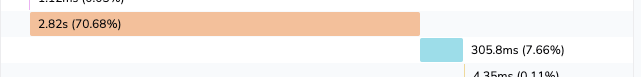
An example of a trace for an abnormally long request before we shipped asynchronous counting: the top trace is the SQL COUNT query, while the query after it is the SELECT query retrieving one page of results.

A way to resolve this issue without compromising too much on the UX is to split the HTTP requests in 2 parallel requests:

1. A request to fetch a page of items
2. A request to fetch the total count

The user is able to look at the results being displayed as soon as request 1 completes, while the total count comes asynchronously later.

Asynchronous counting: The first query retrieves a page of results as rapidly as possible, while a second query is querying the total count for the given filters.

Premium Replication

One thing that greatly affects query performance is the cache of the database. The difference in performance between the query using cold cache vs hot cache can be dramatic. In some examples, we measured 20x better performance between cold and hot cache.

Besides analytics that are served by Snowflake, all our production traffic was served by our primary PostgreSQL instance, meaning that the PostgreSQL cache was shared by all features and all customers (users on our free tier alongside paying customers).

In order to reserve more cache capacity to paying customers using our hottest dashboard views, we created a PostgreSQL replica of our entire database, used exclusively for reading by paying customers and our hottest endpoints.

In addition to providing a smoother experience to customers, this replica also brings a way better isolation against “noisy neighbors”. Indeed, our main dashboard views are now indifferent to potential spikes in database CPU that could come from anywhere else in the app.

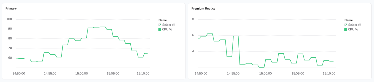
On the left: a heavy process triggers a CPU burst on our primary database instance. On the right, the premium replica used by business customers to access the dashboard hot views is not affected by this burst.

Full-text search optimizations

Our incidents listing view supports full-text search over incidents, on a whole lot of attributes. When examining traces, we saw that the search query string was one of the heaviest contributors to long requests (requests taking more than 3 seconds).

Our text search is powered by the pg_trgm extension, which breaks down strings in all their trigrams, and indexes them against row(s) containing the matching trigram. When searching for text against one of the indexed columns, the search query is again broken down in trigrams, that are then queried using the index.

As we support searching on various attributes linked to an incident, we were encountering two problems:

• Product-wise, the UX was not optimal, because customers had difficulty understanding which attribute of a given item was at the origin of this item matching the search.
• Technically, the underlying SQL query was an UNION statement uniting the results of various queries filtering on different tables.

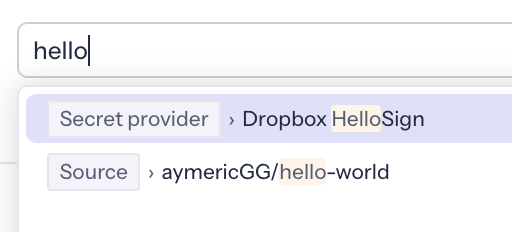
To address those two issues, we overhauled the search experience so that instead of directly returning results, the full text search separately searches the supported attributes, and then allows the user to choose one to filter over.

This approach yields several benefits:

• Users know exactly what they are filtering over
• Searches over several distinct attributes can be broken down in several requests, each of which are faster, and can be requested in parallel.
• The front-end can use local caching to avoid re-requesting the matching attributes for a given query.
• Once users select their intended filter, it’s not a full-text search anymore, as results are being queried based on the specific chosen attribute.

Denormalization

The last angle we explored was optimizing filtering on specific fields for which we noticed anomalous performance in our traces.

By studying query plans, we found that when filtering and sorting a paginated result, PostgreSQL must choose between two strategies:

1. Scan the main table in sort order, apply the filter row-by-row, and stop once N results are found.
2. Use the filter index to find all matching rows up front, JOIN them back to the main table, sort the entire result set, and return the first N elements.

Strategy 1 is efficient when matching rows are frequent in the table: PostgreSQL finds N results quickly. But when the filter is selective, it may scan the entire table before finding enough matches. Strategy 2 handles selective filters well, but degrades when many rows match.

PostgreSQL picks between them using per-table statistics, which is probabilistic. In some cases it chooses the wrong strategy, leading to consistently slow queries for certain filters.

The reliable fix is a composite index covering both the filtering and sorting criteria, allowing the planner to find matching rows and iterate them in order without a separate sort. The catch is that composite indexes must live on a single table, so when the filter field belongs to a related table, it must first be denormalized, either onto the main table, or onto a dedicated denormalization table (we chose the latter).

For example, consider this query, which filters incidents according to the validity of their secrets:

SELECT *
FROM incident i
JOIN secret s ON i.secret_id = s.id
WHERE i.account_id = 42
  AND s.validity = 'valid'
ORDER BY i.date DESC
LIMIT 50;

By denormalizing the secret.validity column alongside the incident date, we can now create the following composite index:

(account_id, validity, issue_date)
 ^^^^^^^^^^^^^^^^^^^^  ^^^^^^^^^^   
 matches filters     | matches ordering

Using this index, PostgreSQL is able to directly match the portion of the index matching the filters, and then scan this index in the sort order, stopping once it has 50 entries.

PostgreSQL 18 upgrade

PostgreSQL-level improvements were also part of this project. In parallel with the application and query changes described above, we upgraded our production stack to PostgreSQL 18. This gave us incremental wins “for free” on some workloads and, just as importantly, put us on a stronger baseline for future performance work.

The key point is that the upgrade was an accelerator, not a silver bullet: the largest gains still came from the targeted changes we made in query design, counting strategy, search behavior, and cache isolation. But running on PostgreSQL 18 helped us stabilize those gains and reduce the risk of regressions over time.

The results

A good sketch is better than a long speech. 👇

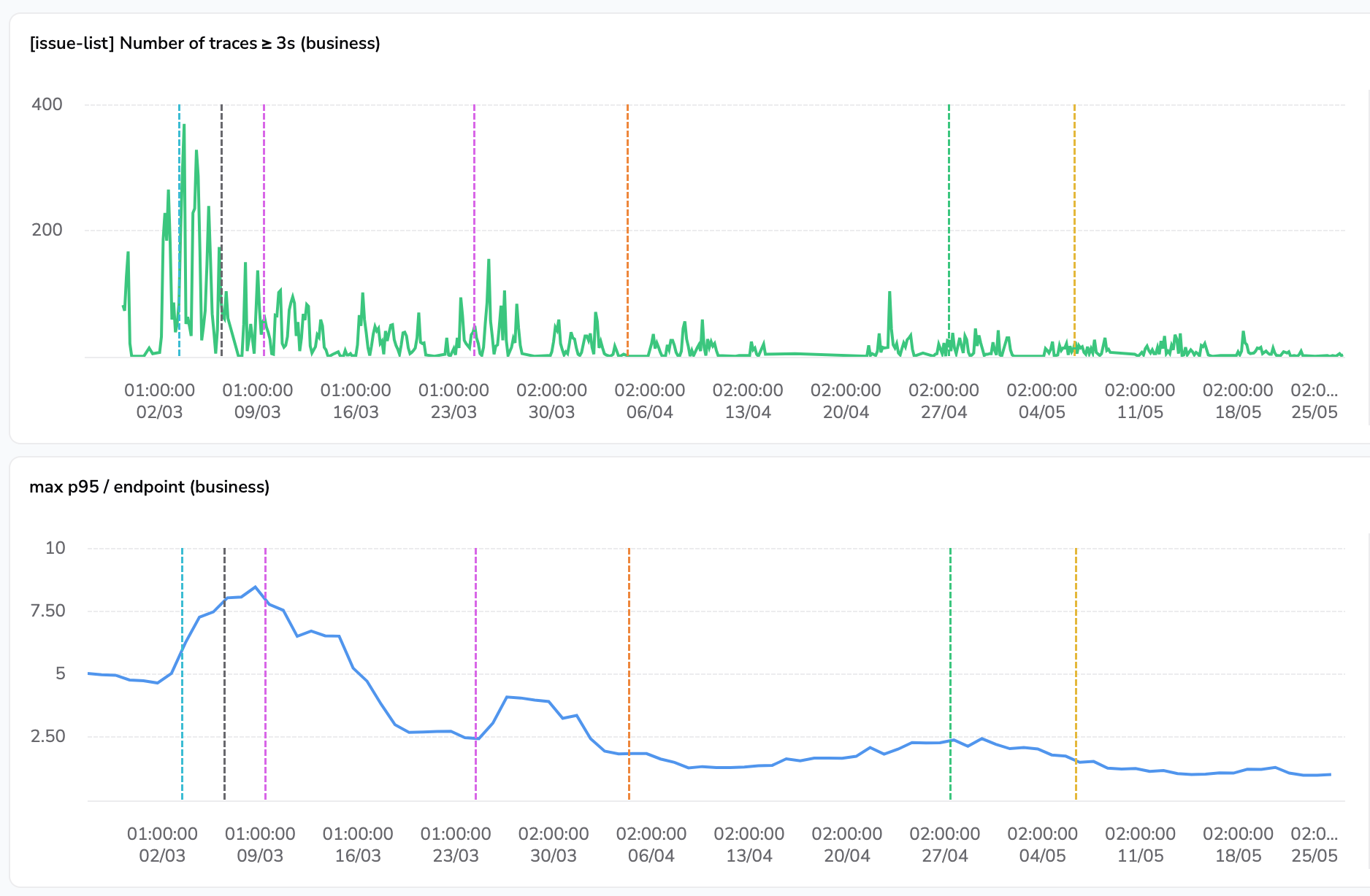
The chart above shows:

1. The number of traces on our hottest dashboard view that are greater or equal to 3s.
2. The p95 of this endpoint for our paying customers.

On the first chart, we can notice groups of 5 spikes separated by flatter segments, which correspond to weeks and week-ends. The second chart is smoothed over a 7-day period to ease the reading of trends. On both charts, vertical annotations correspond to the shipping dates of different parts of the optimizations exposed in this article.

The latest value of p95 at the right of the second chart is 1s, comfortably below our 3-second target.

Conclusion

For customers, the outcome of the project is immediate: faster dashboard interactions, shorter investigation loops, and more consistent performance, even on very large datasets.

On the engineering side, it did more than just reduce latency. We introduced replica-based reads on critical paths to improve isolation from noisy neighbors, redesigned search to be both clearer and faster, and laid practical foundations for further denormalization when it makes sense. Along the way, we also deepened our PostgreSQL expertise across the team.

Just as importantly, this work raised our collective performance awareness: we now have better observability and alerting to catch performance regressions. And while these optimizations already deliver strong gains today, they also de-risk our longer-term path toward a dedicated analytical store with ClickHouse.

Ultimately, this project reflects a core engineering principle at GitGuardian: solving hard technical problems is only meaningful when it translates into a better day-to-day experience for our users.

---